Analytical solutions of SIR models

These notes were written in the early stage of the COVID19 pandemic and they explore general properties of compartmental transmission (SIR-type) models.
The models below make no specific predictions, instead I am only looking at their general mathematical properties.

SIR models

Let’s start with the simplest epidemic model, ie. the SIR compartmental model, where we have:
$\frac{dS(t)}{dt}{=}{-}\alpha S(t) I(t) \\ \frac{dI(t)}{dt}{=}\alpha S(t) I(t)-\beta I(t) \\ \frac{dR(t)}{dt}{=}\beta I(t) \tag{1}\label{SIR_odes}$

It is more convenient to work with fractions of a population (and not absolute numbers), so that we have the conservation $S(t){+}I(t){+}R(t){=}1$. We need to keep in mind that this is a mean field ODE model and has many limitations. It assumes complete homogeneity of transmission events, ie. that they depend only on the fraction of the population susceptible and infected and that for given values of these fractions we have the same rate of transmissions. This also means that any small nonzero values for the infected population will lead to transmissions, whereas in reality a very small fraction can mean so few infected individuals that the epidemic can just die out. Also, in reality transmission events (very probably) do not occur homogeneously, proportionally to the infected (and susceptible) fraction of the entire population, but are much more clustered, local and occurring in certain environments, in burst-like (‘superspreader’) events. For these reasons it is important to stress that these SIR models should be interpreted very cautiously and we must keep in mind their assumptions that are not entirely correct. Nevertheless, they can give us a first idea of some general properties of epidemic dynamics and that’s what I want to do here. For predictions and planning more advanced models that take into account local environments, stochasticity, rare spreading events etc should be used, and it can also be useful to use very simple but probabilistic models.

In the SIR framework it is clear that $I(\infty){=}0$, since this variable has first-order (linear) decay, so any nonzero value in this compartment eventually ‘leaks out’ into $R$. Therefore the equilibrium of the system is $(\overline{S},0,\overline{R})$ and due to the conservation $\overline{R}{=}1{-}\overline{S}$. So to characterize the stationary behavior of the system all we need to calculate is $\overline{S}$.

Of course this can be done by numerically integrating the ODEs in \ref{SIR_odes} and indeed half the internet is full of SIR-models now. But how about an exact solution?
In this very clear paper in Nature Medicine (and probably others before) the authors explicitly derive the stationary solution for a more complicated model of 8 variables they abbreviate as the ‘SIDARTHE’ model. Despite the apparent complexity this model is basically identical to the simple SIR model. The only difference is that 1) the $I$ variable is split into several sub-variables (I: infected, a-/presymptomatic, undetected, D: diagnosed (asymptomatic infected, detected); A: ailing (symptomatic infected, undetected); R: recognized (symptomatic infected, detected); T: threatened (infected with life-threatening symptoms, detected)) 2) the sink variable R of the SIR model is split into two sinks (H: healed (recovered); E: extinct (dead)). However the $IDART$ ‘module’ (the five state variables representing different stages of infection) has the same basic property as I, namely that in $t{\rightarrow}\infty$ they decay to 0, and only S, H, E can have nonzero values.

For the simple SIR model defined of \ref{SIR_odes} the solution for the stationary value of $\overline{S}$ is less complicated than in the latter model, ie. it is given by the implicit expression:
$\frac{\alpha}{\beta} \overline{S} - log\overline{S} = \frac{\alpha}{\beta} - logS(0) \tag{2}\label{SIR_S_stationary}$

This can be solved by an efficient algebraic solver such as $fsolve$ in MATLAB. Let us do a parameter sweep in the $\frac{\alpha}{\beta}$ ratio and the initial value of $S(0)$, and look at the stationary solution of R, ie. the fraction of the population that went through infection (ie. is now immune, if there is long-term immunity). Let us also check if the algebraic formula is the same as integrating the ODEs of \ref{SIR_odes} for a long time span: 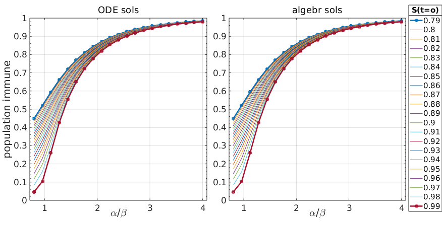Figure 1: Stationary solutions of SIR model calculated by simulations (left) and exact calculations (right)

Fortunately the analytical solutions from \ref{SIR_S_stationary} are identical with the numerical solutions of the ODEs, so we didn’t make a mistake in \ref{SIR_S_stationary}.
What do we see from this plot? The $\frac{\alpha}{\beta}$ ratio is the famous $R_0$, the basic reproduction parameter, and logically, the larger this ratio is, the more of the population will go through infection (again, in the framework of this extremely simplified model not meant to be realistic). It is also intuitive that if $S(t{=}0)$ is smaller because of a larger initial infected population $I(0)$, then $\overline{H}{+}\overline{E}$ will be larger.

Now, let us make the model one step more refined, and split R into two variables, H(ealed) and E(xtinct , ie. deceased), as:

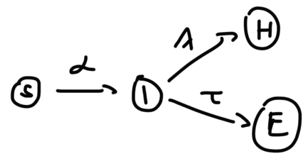Figure 2: ‘SIHE’ version of the SIR model where R(recovered) is split into H and E

The I(nfected) variable now has two outcomes. It is clear intuitively that this will not change how the stationary solution of $\overline{S}$ is calculated, as the sink nodes do not interact with S, except that now I has two outgoing flows, so it is the ratio $\frac{\alpha}{\lambda{+}\tau}$ that will define $\overline{S}$ as: $\frac{\alpha}{\lambda{+}\tau} \overline{S} - log\overline{S} = \frac{\alpha}{\lambda{+}\tau} - logS(0) \tag{3}\label{SIHE_statsol_S}$

Moreover we can give the formulas for $\overline{H}, \overline{E}$ as a function of $\overline{S}$ and the initial infected population $I(0)$. It is reasonable to assume $H(0), E(0)$ are 0. Downstream of I the dynamics is completely linear: what flows out from S into I (ie. $\Delta{S}{=}S(0){-}\overline{S}$), as well as the initial concentration of $I(0)$ will be partitioned into the sink variables proportionally to the rate constants $\lambda$ and $\tau$. Specifically, we’ll have:
$\overline{H} = [(S(0)-\overline{S}) + I(0)] \frac{\lambda}{\lambda{+}\tau}\\ \overline{E} = [(S(0)-\overline{S}) + I(0)] \frac{\tau}{\lambda{+}\tau} \tag{4}\label{SIHE_statsol_H_E}$

The ratio $\frac{\tau}{\lambda{+}\tau}$ is the infection fatality (IFR) rate. It is clear from \ref{SIHE_statsol_S} that the IFR does not affect $\overline{S}$ if the sum $\lambda{+}\tau$ is kept constant, it is instead the ratio of $\alpha$ (rate constant of new infections) to these two parameters that determine at what level of total infections the epidemic stops. To check if the formulas are correct, let us again compare the exact solution to the numerical solution of the ODEs, and plot the stationary solutions of $\overline{S},$ at different IFR values: 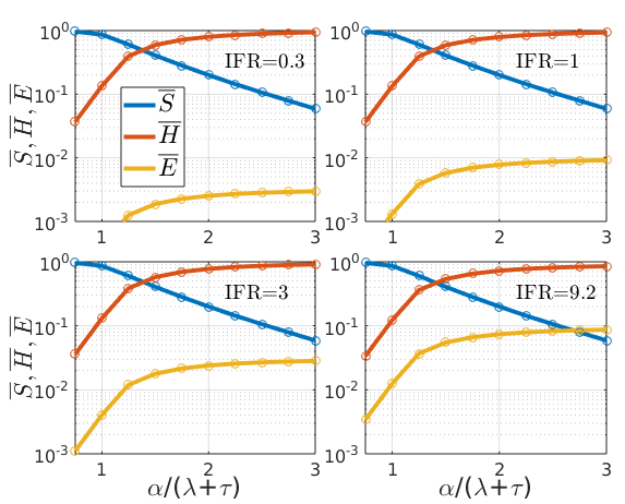Figure 3: stationary solutions of SIHE model at S(0)=0.99 and four different values of the IFR

Circles show the results from numerical integration of the ODEs, confirming they are identical with the analytical solutions (lines). The fraction of the population that has not been infected throughout the epidemic ($\overline{S}$) goes down with $\frac{\alpha}{\lambda{+}\tau}$, but is independent of the IFR as the sum ${\lambda{+}\tau}$ was kept constant here. The ratio $\frac{\alpha}{\lambda{+}\tau}$ expresses how fast subjects exit the infectious state relative to the rate constant of generating new infections. A higher ratio means more of the population is infected, which is $\overline{H}+\overline{E}=(S(0){-}\overline{S}){+}I(0)$. In contrast, if both $\alpha$ and $\lambda{+}\tau$ are equally scaled then this quantity does not change.
How the infected fraction of the population is partitioned between the two sink states ($\overline{H}, \overline{E}$) obviously depends on the IFR (note the logarithmic scale), as stated in \ref{SIHE_statsol_S}. Note that while the IFR is ‘hard-wired’ in the parameter ratio $\frac{\tau}{\tau+\lambda}$, how much of the population gets infected and dies depends on $\overline{S}$ and therefore $\alpha$, the rate constant for transmission. This is where physical distancing measures would intervene to choke off the flow ${S}\rightarrow{I}$.

Let us go now one step further and allow for a pre-symptomatic state, defining I as a variable of the infectious but pre-symptomatic state and adding a variable A(iling) that is the infectious and symptomatic state. Now the compartments of this ‘SIAHE’ model and the flows between them are:

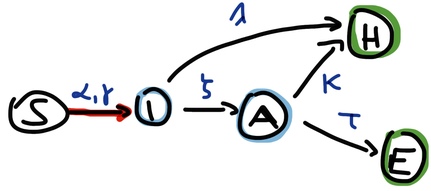Figure 4: ‘SIAHE’ SIR model with presymptomatic (I) and symptomatic (A) infectious state and two outcomes

By highlighting the ${S}\rightarrow{I}$ flow in red I want to indicate that this is the (only) nonlinear term, and now this flow has two parameters as the ODE for S is:
$\frac{dS(t)}{dt} = -S(t)(\alpha I(t) + \gamma A(t))$

These two bilinear terms are positive feedbacks on the otherwise linear system. If it wasn’t for these terms the system would have an equilibrium where only the terminal vertices ($H, E$) of its graph can have nonzero value, just like with the equilibrium we have for the state transition graph of a stochastic Boolean model. Because of this nonlinear feedback however S can (and usually does) also have a nonzero value in steady state, so the equilibrium of SIAHE is $(\overline{S},0,0,\overline{H},\overline{E})$.

Let us again get the formula for $\overline{S}$. Ff we have this, the rest of the system has linear kinetics, so the stationary values of H and E will follow easily from the kinetic matrix of the IAHE variables. I follow here the derivation from the Nature Medicine article, except that it is for a simpler (5 variables) model.

We need to introduce some notation:
$x(t){=}\begin{bmatrix} I(t) \\ A(t) \end{bmatrix}, c{=}\begin{bmatrix} \alpha \\ \gamma \\ \end{bmatrix}, b{=}\begin{bmatrix} 1 \\ 0 \end{bmatrix}, F{=}\begin{bmatrix} -(\lambda{+}\zeta)&{0}\\{\zeta}& -(\kappa{+}\tau) \end{bmatrix}$

Then the ODE for $I(t)$ and $A(t)$ is:
$\dot{x(t)}{=}F x(t) + b c^T x(t) S(t)$

Since $\dot{S}(t){=}-c^T x(t) S(t)$ we can substitute this in and get:
$\dot{x(t)}{=}F x(t) - b \dot{S}(t)$

Then integrating (and changing $t$ to $\phi$), for the left side:
$\int_0^\infty \dot{x}(\phi) d\phi = x(\infty){-}x(0){=}-x(0)$

…and on the right hand side we have:
$F\int_0^\infty x(\phi) d\phi - b \int_0^\infty \dot{S}(\phi) = F\int_0^\infty x(\phi) d\phi - b(\overline{S}-S(0))$

so then we have:
$-x(0){=}F\int_0^\infty x(\phi) d\phi - b(\overline{S}-S(0))$

Now if we pre-multiply by $c^T F^{-1}$ (a [1x2] vector) to get rid of F and to turn both sides into scalars we get:
$-c^T F^{-1} x(0) =\int_0^\infty c^T x(\phi) d\phi - c^T F^{-1} b(\overline{S}-S(0))$

From the ODE of $\dot{S}$ we can substitute $\frac{\dot{S(t)}}{S(t)}$ into $c^T x(t)$:
$-c^T F^{-1} x(0){=} - \int_0^\infty \frac{\dot{S}(\phi)}{S(\phi)} d\phi - c^T F^{-1} b(\overline{S}-S(0)) = log \frac{S(0)}{\overline{S}} - c^T F^{-1} b(\overline{S}-S(0))$

Then after a rearrangement we have the solution for $\overline{S}$ in the same form as for the ‘SIHE’ model in \ref{SIHE_statsol_S}:
$-c^T F^{-1}b \overline{S} - log \overline{S} = -c^T F^{-1}b S(0) - log S(0) + c^T F^{-1} x(0)$

$-c^T F^{-1} b$ is the $R_0$ of this version of the model, so rewriting with $R_0$:
$R_0 \overline{S}- log \overline{S} = R_0 S(0) - log S(0) + c^T F^{-1} x(0) \tag{5} \label{SIAHE_S_statsol_R0}$

Explicitly, $R_0$ is:
$R_0{=}\frac{\alpha}{\lambda+\zeta}{+}\frac{\zeta \gamma}{(\kappa+\tau)(\lambda+\zeta)}$

$R_0$ is linearly increasing in the contagion rates $\alpha$ and $\gamma$, while decreasing in the rate constants of the outgoing flows of I and A, ie. $\kappa, \tau, \lambda$. $\zeta$ has a more complicated effect as it decreases the first term, but increases the second. This makes sense too, since this is the rate constant between the two contagious states I and A.

Written on April 18, 2020

[ epidemics  complex-systems  covid19  ]