A toy model of dynamic prices of production

I have not posted lately on A. Trigg’s book on reproduction schemas as I got into reading on the (in)famous ‘transformation problem’ and could not resist playing with some models in the literature. In one sentence the transformation problem is about whether the claim that the value of commodities is indirectly or directly determined by the average labour time needed for their production (+ non-labour inputs) is compatible with the observation/expectation that profit rates across sectors with different labour/capital ratios would tend toward equalization. I will not discuss this problem per se in this post, there is a lot of literature available on that, although this model can be regarded as a solution to the ‘transformation problem’. I want to write down the equations of a dynamical model proposed in Kliman [1988] with numerical examples (but without the equations explicitly), of prices of production where the aggregate equalities (total price) = (total value) and (total surplus value) = (total profit) are satisfied, total supply can be sold in each period of production, and the balancing condition (see Eq. \eqref{balancing_cond}) between the two sectors of the economy is also met. The model has the following assumptions and properties:
1) value is expressed in money, there is only one accounting system
2) non-labor inputs transfer their value to the products they are used up for, but no more or less
3) a given amount of labor adds the same amount of value, profit can therefore originate only from unpaid (surplus) labour: less is paid for wages than the amount of new value added by labour, the difference between the two appears as profit (for the entire economy, not for an individual sector)
4) the system shows simple reproduction only: it is producing the same physical amounts of goods in each period, and the physical surplus (output minus inputs used up) takes the form of consumption goods only and it is consumed in each period instead of being redirected (accumulated) into the system as new capital goods or new consumption goods for an expanding workforce. The amount of non-labour inputs (constant capital) and work performed do not change.
5) the real wage is kept constant: the wage paid for workers enables them to buy the same amounts of consumption goods. The nominal wage can however change if the unit price of consumption goods change.
6) Profit rates are equalized

Of course assumptions no. 2-3 can be (are) contested, and the idea that human labour is the only source of new value and therefore of profit can be rejected, but this - ie. the validity of the labour theory of value - is a topic for another post. Assumption no. 4-5 are just convenient first assumptions, but the system can be changed to expanded reproduction etc. by altering its coefficients. Assumption 6 is reasonable as a tendency (capital flows in search of (sectors with) higher rates of return) but one should also have a mechanism implemented in a more serious model. My goal here is just to build a small mathematical model that is internally consistent and has a dynamics that can later be made more realistic by introducing more detail. As the system is dynamic prices and profit rates can change, which is a precondition to incorporate crises in the model.

Like in the input-output models I discussed previously we have two economic sectors (or departments), the first ($D_1$) producing capital goods (this could be raw materials as well, any non-labour inputs used up in production), the second ($D_2$) consumption goods (CoG). Since we are dealing with simple reproduction and we will also abstract from fixed capital, therefore all capital goods are used up in each period of production, the total use of capital goods has to equal the total output ($W_1$) of $D_1$. This gives us the equality $W_1 = C_1 + V_1 + S_1 = C_1 + C_2$, or,
$C_2 = V_1 + S_1 \tag{1}\label{balancing_cond}$ In other words, the exchanges between the two departments (wages + profits in D1 = value of constant capital used up in D2) have to be equal.

In one important respect the current model will be different from the one discussed in the case of input-output tables and this will change the meaning of the equality of Equation \eqref{balancing_cond}. In the input-output description it is assumed (this assumption can be called ‘simultaneous valuation’) that unit prices for the two goods have to be the same when they enter as inputs and when they emerge as outputs in a given period of production. Since unit prices cannot change what the system describes are the relative prices required to solve the system of algebraic equations that describe the input-output equalities. A uniform profit rate is normally assumed, which gives one more constraint for the price system, but since there is one more unknown than the number of equations, only relative prices can be calculated. The input-output model as usually understood is then a model of equilibrium prices for given technical (input-output) coefficients and a level of real wage (units of CoG paid for a unit of labour performed). In fact, because of the fact that input and output prices are the same and that profit rates are equal across sectors, both prices and the rate of profit are determined by the technical coefficients and the real wage rate (which is also a physical quantity), and in a sense prices become irrelevant (see Kliman (1999)).
In contrast, in the model I will discuss here this assumption of the equality of input and output unit prices is dropped: input prices determine output prices sequentially. Consequently, instead of a system of algebraic equations with the same unit prices on both the right and left side, we will have a system of difference equations, that we need to provide with initial values in the first period of reproduction. In periods t>1 the input prices are given by the output prices of the preceding period.

To summarise, in the simultaneous description we have unit prices as: $\mathbf{p} = \mathbf{p}(\mathbf{A} + w \mathbf{l})(1+r) \tag{2}\label{simul_val}$

where $\mathbf{p}$ is the row vector of unit prices, $\mathbf{A}$ the input-output matrix, $w$ is the wage rate, $\mathbf{l}$ is the row vector of labour inputs (quantities) per unit of output of each commodity and $r$ is the profit rate. $\mathbf{A}$, $w$ and $l$ are given, whereas $\mathbf{p}$ and $r$ are the unknowns. Defining the ‘augmented’ input matrix $\mathbf{M} = A + w l$, we can write the profit rate $r = (pX - pMX)/pMX$, where X is the column vector of gross outputs (physical quantities), but this is not an independent equation but rather comes from $\mathbf{p X} = (\mathbf{p} \mathbf{M} (1+r))\mathbf{X}$, so although $r$ can be calculated (given $\mathbf{M}$), but for production prices $\mathbf{p}$ we will only have the relative prices, as any set of absolute prices with the same ratios will satisfy the equations.

In the dynamic description we have instead: $\mathbf{p}_{t+1} = \mathbf{p}_t(\mathbf{A} + w \mathbf{l})(1+r) \tag{3}\label{dynamic unit prices}$ which is a system of difference equations, not algebraic ones. Here, the input unit prices are a given, they are data, and they are mapped onto the output prices by the technical coefficients, the wage rate and the markup of the aggregate profit rate. Moreover, because of the third assumption above, the profit rate can now be independently determined from the input unit prices, technical coefficients, the wage rate and the amount of labour performed: $r_{t,t+1} = (\mathbf{l}\mathbf{X} - \mathbf{p}_t w \mathbf{l} \mathbf{X})/ (\mathbf{p}_t (\mathbf{A} + w \mathbf{l}) \mathbf{X}) \tag{4}\label{profit_rate_dynamic}$

Profit is the total amount of new value added minus the real wage of workers (quantity of consumption goods times their input unit price). The rate of profit is given by dividing the amount of profit by total input costs that are also defined by technical coefficients, the wage rate and the input prices. It can be seen that the calculation of the profit rate only involves the input data of input prices and the coefficients, therefore it comes first. The calculation of unit output prices follows after, since they are the function of both the profit rate and input prices as can be seen from Equation \eqref{dynamic unit prices}.

Now let us go back to the equality of simple reproduction in Equation \eqref{balancing_cond}:
$C_2 = V_1 + S_1$ (coming from $W_1 = C_1 + C_2$, $W_i$ being gross output of a sector)
In the equilibrium description of input-output tables, where input and output unit prices are equal, this equality is a relation between the inputs and outputs of the same period. As this is a description of equilibrium for a given set of technical and wage coefficients, there is in fact only one period, if we take another set of coefficients then we need to calculate another set of equilibrium prices. But in the dynamic description this balancing condition is across two periods: the output of one period is the input of the next. In price terms, the output of capital goods has to equal the input of capital goods in the next period. In physical terms, since it is simple reproduction, it is also true that the inputs (of one good) used up in the current period has to equal the output (of the same good) of the current period. But in terms of money the current period’s output is the input of the next one, and it does not need to equal the input of this period, unless the difference equations for unit prices have reached their stationary value. So the equality in the dynamic setting will be: $W_1(t) = C_1(t+1) + C_2(t+1)$.

Let us write the dynamic equations for the unit prices in a form that they contain no other time-dependent variables, but only constants. All other variables of the system are governed by the unit prices as follows (from now on I put the time index in parenthesis instead of a subscript, as I use subscripts for department indices):

• constant capital: $C_1(t) = \alpha X_1 p_1(t)$, $C_2(t) = (1-\alpha) X_1 p_1(t)$, since the total physical amount and sectoral distribution of capital goods do not change
• wages: $V_1(t) = \beta_1 X_2 p_2(t)$, $V_2(t) = \beta_2 X_2 p_2(t)$, since the real wage is defined as a fixed amount ($\beta_1$, $\beta_2$) of consumption goods ($X_2$) that the wages can buy, and distribution of the workforce does not change
• revenue: $m(t)=\mu X_2 p_2(t)$, profit spent on consumption goods by capitalists, also kept constant in physical terms ($\mu X_2$, and $\mu + \beta_1 + \beta_2 = 1$)
• total (gross) output: $W_i(t) = p_i(t) X_i$
• cost: $K_1(t) = C_1(t) + V_1(t) = \alpha X_1 p_1(t) + \beta_1 X_2 p_2(t)$, $K_2(t) = (1-\alpha) X_1 p_1(t) + \beta_2 X_2 p_2(t)$
• profit rate: $r(t) = \frac{L_T - (V_1(t)+V_2(t)) }{ K_1(t) + K_2(T)} = \frac{L_T - (\beta_1 + \beta_2) X_2 p_2(t)}{ p_1(t) X_1 + (\beta_1 + \beta_2) X_2 p_2(t) }$ ($L_T$ is total labour performed)

Since the output price of the current period is the input of the next period, and gross output is equal to input costs and a markup equal to the aggregate profit rate, we have: $p_i(t+1) X_i = W_i(t) = (C_i(t) + V_i(t)) (1 + r(t)) \tag{5}\label{unit_price_dynam_implicit}$

Dividing by $X_i$ and substituting the expressions listed above we have:
$\begin{bmatrix} p_1(t+1) \\ p_2(t+1 )\\ \end{bmatrix} = \begin{bmatrix} \alpha & \beta_1 X_2 / X_1\\ (1 - \alpha) X_1 / X_2 & \beta_2 \\ \end{bmatrix} \begin{bmatrix} p_1(t) \\ p_2(t)\\ \end{bmatrix} \frac{ p_1(t) + L_T/X_1 }{ p_1(t) + (\beta_1 + \beta_2) X_2/X_1 p_2(t) } \tag{6}\label{unit_price_dynam_explicit}$

This is a system of first-order, non-linear, autonomous difference equations, that - I think - cannot be solved analytically (so that $p(t)$ would be a function of time and parameters only), but it is easy to simulate numerically, or solve for its fixed point (in which case it becomes a quadratic equation, with one positive solution).

I simulated the system in MATLAB with the following numerical values (also used in the article cited below as a reference): $L_T = 300$, $\alpha = 1/2$, $\beta_1 = 1/6$, $\beta_2 = 1/3$, $\mu = 1/2$, $X_1 = 200$, $X_2 = 300$ and the initial values $p_1(0)=p_2(0)=1$. This is the plot of the dynamics of unit prices and some of the ratios of the system:

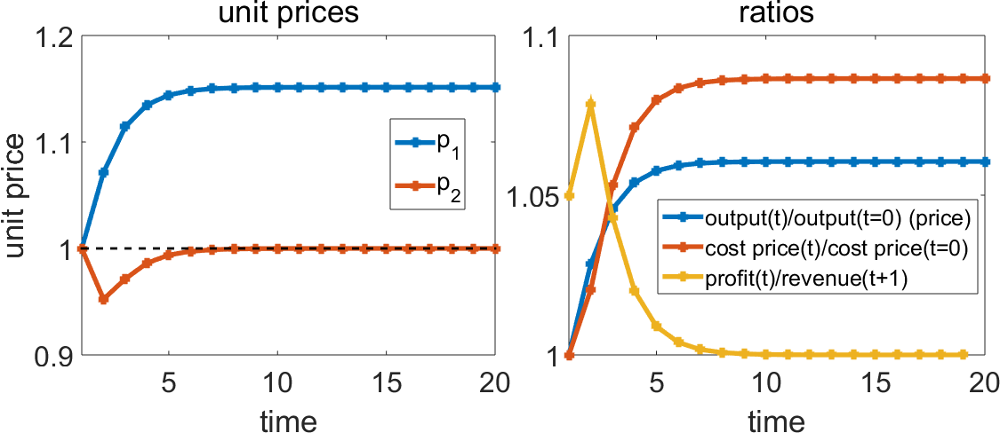
The system satisfies the following equalities (these are all in price terms):

• $W_1(t) = C_1(t+1) + C_2(t+1) = p_1(t+1) X_1$, output of capital goods of the current period equals input of capital goods in next period
• $m_1(t) + V_1(t) = C_2(t)$, exchanges between the sectors have to balance (capitalist consumption + wage outlays from $D_1$ equals outlays on capital goods from $D_2$, with the other transactions being within the two departments)
• $W_2(t) = V_1(t+1) + V_2(t+1) + m(t+1) = p_2(t+1) X_2$, output of consumption goods in current period equals outlay on wages plus consumption from profit (revenue) in next period
• $\sum m_i(t) = \sum W_i(t-1) - \sum K_i(t)$, total revenue, ie. profit that can be spent on consumption equals the difference between the output of the previous period minus outlays on wages and capital goods in the current period

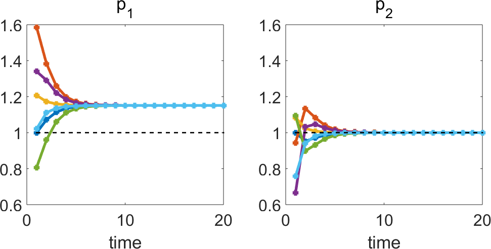
Since unit prices are changing until we reach the stationary state, the amount of money needed for total outlays (wages + capital goods) is also changing (see on the plot above the ratio of costs), and since inputs (in this model) transfer their prices to the output, gross output in terms of price is also changing, though net value added does not. Once we reach the fixed point unit prices do not change anymore, therefore wages, profit, outlays on capital goods and gross output have also reached a stationary state. This final state is identical to the equilibrium price (equal input and output prices) solution to the system. The fixed point is obviously attracting, so sampling in initial values (for unit prices) will lead to the same stationary values, as shown in the plot below.

But the dynamical system converges to this stationary state only because the technical coefficients, the physical productivity and relative sizes of the departments do not change in this model. If the parameters change before the system converges to the fixed point, then the pre-equilibrium behavior will continue (see Giussani 1991). This simple model satisfies the requirements of a labour theory of value that total profit equals total surplus (unpaid) labour, total price equals total value, and the sectoral balances of simple reproduction are also respected, although this is enforced by the assumptions of the model that I’ll mention below. The unit prices of the two goods are different from their values, so it is only through aggregate quantities that prices are determined by labour values.

If we want to add additional detail to the model, the first thing to add should probably be growing labour productivity that would also mean expanded reproduction, so that some of the surplus is recycled to the system and not consumed. The other component to add for a bit more realistic model is fixed capital. If we add these, then it can start to make sense to ask questions on how productivity growth will affect profitability.

There are several potential problems with this model. First is how can we know the amount of value a unit of labour adds or represents, and the assumption that this amount (the ‘monetary expression of labour time’) does not change. The second is that non-labour inputs (there is only one type in this model, ‘capital goods’ in general) transfer the value that they were bought at, but what happens if due to changes in productivity the inputs are worth less when the production period comes to its end, than at their time of purchase, what amount of value would they transfer? Third, nominal wages automatically adjust to the new price of wage goods, as wages are defined as a fixed physical amount of wage goods times the output price of the previous period, assuming perfect adjustment of wages to match the supply of wage goods. Finally, since the price of total output is growing, there needs to be more money in the system then in the first round (with the coefficients and the initial values used above), so the money supply would have to expand. I will return to these problems in future posts.

Script

MATLAB script

References

Giussani: The Determination of Prices of Production, International Journal of Political Economy, Volume 21, 1991
Kliman, McGlone: The transformation non-problem and the non-transformation problem, Capital & Class, Vol 12, Issue 2, 1988
Kliman, McGlone: A Temporal Single-system Interpretation of Marx’s Value Theory, Review of Political Economy, Volume 11, Number 1, 1999

Written on January 12, 2019

[ political-economy  economic-models  classical-political-economy  marxian-economics  transformation-problem  nonlinear-dynamics  ]