The monetary circuit (I)

In the previous post I discussed the so-called ‘Kalecki’ principle, which, in my understanding, is an equality between gross profits on the one side and spending on capital goods and capitalist consumption on the other, summarized in the phrase ‘capitalists earn what they spend’. This statement implies a causal relationship, which - it seems to me - is not demonstrated by these algebraic relationship. To show that this spending creates (enables/leads to) these profits, one needs a sequential (dynamic) description of how the initial amount spent circulates through the economic system.

A framework to do this is the so-called monetary circuit. The theory of the monetary circuit was developed by A. Graziani and others and shows how an initial injection of money circulates through the economy and return back to the owners of businesses and how much money is needed to close the circuit completely, with all output sold. In the model by Graziani there is a distinction between workers, capitalists and banks. Banks give credit to firms, so they can finance their outlays on wages, since this step has to precede production and sale. Money in this model is credit money, that has symbolic value, but no intrinsic value, ie. it is not a commodity. The starting point of the circuit is banks giving credit to firms to hire workers, who then produce commodities. Assuming that workers don’t save, wages are spent on consumer goods (CoG), returning the money to firms. As the last step of the circuit, firms can then repay their debts, destroying the credit money they originally borrowed and the circuit is closed.
So the circuit is simply: banks –> firms –> workers –> firms –> banks.

In this description it is only wages that have to be advanced by companies, as it does not concern itself with the purchase of capital goods, that is considered to be internal to firms. For this reason I find this description too restrictive and almost tautological. For me, the main problem is to show how the entire output can be ‘realized’ (purchased by money), even if there is an increment of the capital stock and/or the labour force (extended reproduction) and not all surplus takes the form of CoG (consumption goods) that are consumed by owners at the end of the period of production. Starting from a two-sector model and output grouped into gross wages and gross profit we can draw up the following table:

Departments	Wages ($V_i$*)	Profits ($P_i$*)	Output $W_i$
$D_1$ (MoP)	$V_1$*	$P_1$*	$W_1$
$D_2$ (CoG)	$V_2$*	$P_2$*	$W_2$

Table 1: Two sectors, gross profit

If we subsume capitalist consumption under wages (and there is no government sector or foreign trade), then the surplus of the CoG sector ($P_2$) matches the wage bill of the capital goods sector, ie.
$P_2^* = V_1^* \tag{1}\label{p2_equals_v1}$

If in this model only wages are advanced, then the sum of advanced money equals the output of the CoG sector: $M = V_1^* + V_2^* = P_2^* + V_2^* = W_2 \tag{2}\label{advanced_wages}$

But in this case it would seem there is not enough money to buy up the entire output, the capital goods sector does not have the funds to reimburse the banks and the circuit cannot be closed. A simple answer to this is a ‘single swap’ approach (Nell, 2004), that a larger sum $M=W_1+W_2$ is advanced, so that all output can be bought up in a single monetary circuit. But this makes things too easy, resulting in the buildup of extra funds in the capital goods sector when it receives revenue from the consumer goods sector equal to its wage bill, but it also borrowed that amount from banks. Putting aside this too general assumption, EJ Nell (2004) worked out one solution based on multiplier effects within departments, that I discuss next.

Nell’s solution: realizing the total output through multiplier effects

The ‘single swap’ solution just mentioned leaves no place for transactions taking place sequentially, with a given amount of money that is smaller than $M$, circulating between households (workers and capitalists as consumers) and firms in the two sectors. The ‘mutual exchange’ between sectors is key, as firms earn income by selling outputs to firms in the other (and in the same) sector. EJ Nell (2004)’s solution based on mutual exchanges starts with the following assumptions:

• Production is defined in distinct periods.
• In each period of production all capital goods are completely used up (100% depreciation).
• Consumption and capital goods are both carried forward from the previous period, so that at the start of the period, there are inventories of capital and consumption goods ‘inherited’ from the previous period
• Production in the current period is to replace items (CoG and MoP) used up by firms and consumers in the current period

The starting point in this model is the advance of wages in the capital goods sector ($D_2$), but it could be the consumer goods sector too, the point is just to initiate the process. This injection of money then circulates through the system in a sequence of stages, ‘realizing’ (enabling the purchase of) the output:

• Stage 1: $D_1$ borrows money from banks, pays wage bill to workers of $D_1$. Workers spend this money to purchase consumption goods from $D_2$
• Stage 2: After selling consumption goods to workers of $D_1$, $D_2$ pays wages to its own workers, who spend it on CoG, so that the money returns back to $D_2$, to be spent on capital goods from $D_1$.
• Stage 3: From the sales of MoP to $D_2$, $D_1$ firms can advance wages and purchase their own capital goods.

Schematically, the sequence is:
banks -(0)-> $D_1$ -(1)-> $D_1$ workers -(2)-> $D_2$ -(3)-> $D_2$ workers -(4)-> $D_2$ -(5)-> $D_1$ -(6)-> $D_1$ & $D_1$ workers $\tag{3}\label{v1_sequence}$

Now we can see a causal multiplier effect, as the initial injection of money as advanced wages by $D_1$, $V_1$, leads to the realization of commodities of a (multiple times) higher total value. $V_1$ CoG is sold in step (2), then again $V_2$ of CoG in step (4), and $P_1$ (?) of MoP sold in step (5), and more MoP in step (6) when firms in $D_1$ buy MoP from firms within their sector. The flow of money can be seen on this figure I created:

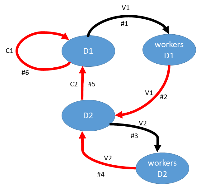
Figure 1: the flow of money through both departments

The red arrows are transactions where a part of the output is ‘realized’ (purchased).

Total money output is:
$W_T = V_1^* + V_2^* + P_1^* + P_2^* = 2 V_1^* + V_2^* + P_1^* \tag{4}\label{total_money_output}$

Nell (1998) describes a multiplier relationship of the wages paid out in $D_1$ on the wages of $D_2$: in the first round this effect is $V_1^*$, then $w n_2 V1^*$, then $(w n_2)^2 V1^*$, with $n_2$ being the labour coefficient (share of labour in total output) and $w$ the wage rate, so that, as $w n_2 < 1$:

$V_2^* = V_1^* \sum_{i=0}^\infty (w n_2)^i = \frac{1}{1 - w n_2} V_1^* \tag{5}\label{v1_v2_multiplier}$ One thing not clear to me is why one would say that in the first round $D_2$ pays out $V_1^*$ as wages, and only from the second $w n_2 V_1^*$, and in later cycles $i$ always $(w n_2)^i V_1^*$.

Nell also assumes two subsectors in $D_1$ (capital goods sector), the first selling MoP to $D_2$, the second to other firms in $D_1$, let us call these $D_{1,2}$ and $D_{1,1}$ (and assume equal labour coefficients and wage rates). A multiplier effect occurs in the exchanges between the subsectors and $D_2$. First, $D_{1,2}$ sells MoP to $D_2$, receiving $P_2^* (=V_1^* )$. It uses $w n_1 P_2^*$ to pay back its loans (if this is not for wages, why the scaling with $w n_1$?) and $(1-w n_1)P_2^*$ to buy MoP from $D_{1,1}$.

$D_{1,1}$ spends $(1-w n_1)(1-w n_1)P_2^*$. But if this is sales within $D_{1,1}$, then the cycle would stop here, whereas Trigg (summarizing Nell) writes that there is a multiplier effect here again, with the sum:

$$P_1^* = P_2^* \sum_{i=0}^\infty (1 - w n_1)^i = \frac{1}{w n_1} P_2^* \tag{6}\label{p1_p2_multiplier}$$

It seems to me, to have this multiplier effect, firms of $D_1$ should use their proceeds to pay back their loans only in the last cycle, before that the mutual exchanges within $D_1$ need to repeat until convergence as in \eqref{p1_p2_multiplier}. In fact, we need to assume that $D_{1,1}$ receives back its own capital expenditure $(1-w n_1)(1-w n_1)P_2^*$, repeating this cycle until convergence and only then spending it, together with $w n_1 (1-w n_1) P_2^*$ on wages, so in total we have $(1-w n_1) P_2^*$ of wage outlays from $D_{1,1}$. I show the multiplier of $D_1$ in this model as I understand it on Figure 2 below.

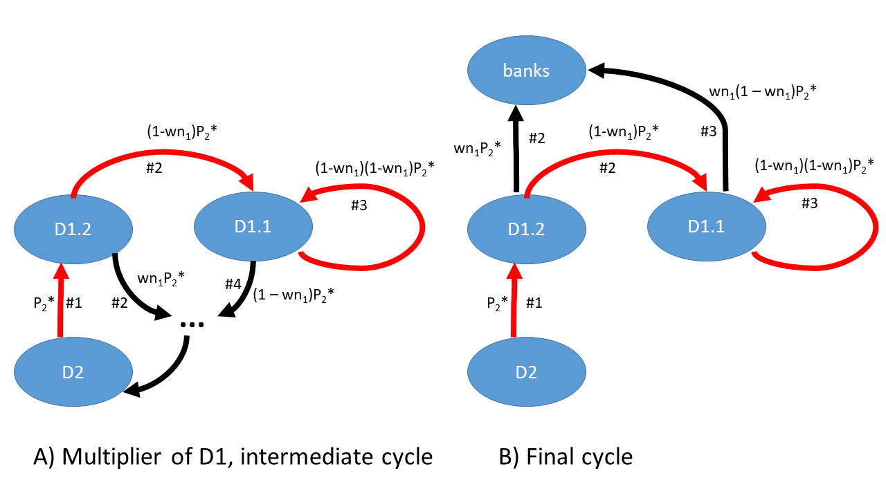Figure 2: the multiplier of $D_1$

It is the two ‘auto-loops’ (to borrow a term from systems biology) within the sectors that generate the multiplier effect. One is the circulating of wages within $D_2$ through its workers: in each round $D_2$ pays wages to its workers that they repay for the same amount of consumption goods. In each round the revenue returned is scaled by $w n_2$ when paid out as wages, which means that the total amount paid out as $V_2^*$ wages (and total amount of consumption good sold within the sector) is $V_1^* \sum_{i=1}^\infty (w n_2)^i = \frac{w n_2}{1 - w n_2}$.

Similarly, within $D_1$ there is first the payment from $D_{1,2}$ to $D_{1,1}$ of $(1-w n_2) P_2^*$, then $D_{1-1}$ buys MoP from itself in a sequence, multiplying the initial amount with $(1-w n_2)$ in each step so in total $V_1^* \sum_{i=1}^\infty (1 - w n_1)^i = \frac{1 - w n_1}{w n_1} = \frac{1}{w n_1} - 1$. So to me it seems the multiplier expressions should be slightly different.

If we substitute the multiplier expressions as in Equation \eqref{v1_v2_multiplier} and \eqref{p1_p2_multiplier} into Equation \eqref{total_money_output} we get an overall multiplier relationship:

$$W_T = 2 V_1^* + \frac{1}{1-w n_2} V_1^* + \frac{1}{w n_1} V_1^* = V_1^* \left(2 + \frac{1}{1-w n_2} + \frac{1}{w n_1} \right) \tag{7}\label{total_money_output_multipl}$$

In my own calculation this should rather be:

$$W_T = V_1^* \left(2 + \frac{w n_2}{1-w n_2} + \left(\frac{1}{w n_1}-1 \right) \right) = V_1^* \left(\frac{1}{1-w n_2} + \frac{1}{w n_1} \right) \tag{8}\label{total_money_output_multipl_corr}$$

I think this is the correct expression, because if we take equation \eqref{total_money_output_multipl}, and consider that $w n_i = V_i^* /(V_i^* + P_i^* )$ and $V_1^* = P_2^*$ then we have

$$2 V_1^* + V_2^* + P_1^* = 2 V_1^* + \frac{1}{1-w n_2} V_1^* + \frac{1}{w n_1} V_1^*$$ $$V_2^* + P_1^* = \frac{1}{1 - V_2^* /(V_2^* + P_2^* ) } V_1^* + \frac{V_1^* + P_1^* }{V_1^* } V_1^*$$ $$V_2^* + P_1^* = \frac{V_2^* + P_2^* }{ P_2^* } V_1^* + V_1^* + P_1^*$$ $$0 = P_2^* + V_1^* ,$$

which cannot be true. Therefore I think the formula in \eqref{total_money_output_multipl_corr} is the correct one.

The point of this model was to show that the initial outlay of $V_1^*$ is sufficient to fund a much larger total income (wages and profits) in both sectors. At last, we can see a chain of causation behind the algebraic relationship of a multiplier. The simple answer to how it is possible to realize the total output is by the circulation of money between and within sectors, including the circulation between firms and their workers. A substantially smaller monetary advance than the value of the total output circulates through the system multiple times, enabling the transactions through which the entire output can be sold. To see how this happens exactly cries out for a dynamic model, probably using difference equations. (As a first approximation, we can just use a spreadsheet where rows stand for time points (stages) and columns the inventories of commodities and money held by the departments, workers and capitalists.) To be able to realize the full output $W_T$ the $D_1$ -> $D_2$ and $D_2$ -> $D_1$ transactions should occur only once, whereas for the two intra-department multiplier effects to converge these refluxes of money need to happen infinitely many times. Are these assumptions reasonable? This requirement could be relaxed by starting the circuit with a bigger initial outlay than $V_1^*$. A somewhat confusing aspect of this model is why gross wages are paid as the initial outlay, not just $V_1$, as the expansion of the workforce by $dV_1$ should happen only in the next period.

The question that this model tries to answer is not identical with the ‘Marxian’ realization problem, although very similar to it. Here a production period starts with the two departments having inventories of MoP and CoG inherited from the previous period, but no money, and the question is whether all inventories can be sold, and if yes, what initial amount of money is required to do so. If inventories are sold, then production can take place and a supply of new commodities is produced, that will have to be realized in the next period of production, where the same realization problem has to be solved. Notice that in this description production and specifically the production of surplus value is not explicitly addressed, or it is obscured in the gross profit category. Also, there is in fact many cycles of production and sale, but initially I wanted to have a model of a single cycle of production and sale that is closed (everything can be sold).

The other way to look at the problem is to say that firms (and owners as consumers) have funds at the starting point, which they use to buy from the inventories of MoP (inherited from previous period) and (through wages) the inventories of CoG that are available at the start of production. Production takes place and the supply of new products have a higher value (surplus value added by labor over paid wages) than the initially spent amount on wages and capital goods - how can it be bought up? In this second formulation, the concept of the production of surplus value is embedded. It is this formulation of the problem that I turn in the next post.

Reference

Andrew Trigg, Marxian reproduction schema: money and aggregate demand in a capitalist economy. Routledge, 2009

Written on November 18, 2018

[ political-economy  economic-models  marxian-economics  demand  monetary-circuit  ]