Generating multistability by coupling self-activating genes

In this post I want to explore how we can generate a regulatory system that has several (more than 2) fixed points by coupling self-activating genes. It is an expanded model of a toggle switch [1]: two genes (variables) that inhibit each other but also have nonlinear self-activation. The scripts I wrote in MATLAB define a highly abstract, ordinary differential equation (ODE) model that does not describe stochastic fluctuations or the details of the underlying biochemical processes (transcription, translation, folding etc), as my interest here was to model multistable behavior in general.

My idea (coming from this [2] paper) was that if the genes are bistable on their own then their nullclines can have 9 intersection points, ie. the two-dimensional systems when these genes are coupled can have up to 4 stable fixed points. Imagine two ‘S’ letters, one aligned with the $x$ axis, the other with the $y$ axis - how many times can they intersect?

In the main script multistable.m we can first experiment with the parameters of a single self-activating gene: the cooperativity parameter ($n$), the threshold of activation ($K$) and the rate of basal activation (transcription/translation) of the gene ($\mathbf{\beta}$). The ODE for a single gene is:
$\frac{dx(t)}{dt} = \beta + \frac{x(t)^n}{x(t)^n + K^n} - x(t) \tag{1}\label{ode_autoact}$

While I am not assigning specific units to the variables and parameters, it is interesting to note what their dimensions are.
The differential equation describes a rate, a change of concentration (mass per unit of volume) per unit of time, so it has to have a dimension of $CT^{-1}$ (C: concentration, T: time).
$\beta$ also has dimension of $CT^{-1}$. The state variable $x(t)$ refers to the concentration of the gene product so its dimension is $C$ (concentration) and $K$ must have the same dimension.
Then, strictly speaking the second term is dimensionless and would need to have a rate constant with dimension of $CT^{-1}$ and the last term a rate constant with dimension of $T^{-1}$.
Since in practice these parameters only scale the production and degradation processes I am dropping them. This could be interpreted, if we are keen on dimensional consistency, as assuming their value is one, or that all other terms were divided by them.

We choose the values of these parameters as, for example:

k_val=3/4; % threshold (50% of maximal rate)
beta_vals = [0 1e-3 linspace(0.01,k_val,100)]; % range of values for basal rate
n_vals=[2:5 8 10]; % % range of values for cooperativity

We then run the calculation by calling the function fcn_bistab_roots:

[roots_real_nonnegat_matr,roots_all] = fcn_bistab_roots(beta_vals,n_vals,k_val);

Since I am solving here only for the stationary solution (steady state, fixed points) I am not numerically solving the ODE. Instead, within fcn_bistab_roots, I solve eq. \ref{ode_autoact} by setting the left hand side to 0 and rearranging the equation into polynomial form, which is:
$x (x^n + K^n) - \beta (x^n + K^n) - x^n = x^{n+1} - (1 + \beta) x^n + K^n x - \beta K^n = 0$

$x$ here stands for the stationary value of $x(t)$. I solve this polynomial with MATLAB’s root-finding algorithm $root$. There cannot be more than 3 real and nonnegative roots of this polynomial, these physically relevant roots are contained in the matrix roots_real_nonnegat_matr for the parameter sets we generated.

I wrote two functions to visualize the solutions as a function of the basal production rate $\beta$. With fcn_plot_bifurc_diff_n_heatmap we can visualize the results as heatmaps on separate subplots for the different values of the nonlinearity (cooperativity) parameter $n$:

fcn_plot_bifurc_diff_n_heatmap(beta_vals, n_vals, k_val, roots_real_nonnegat_matr)

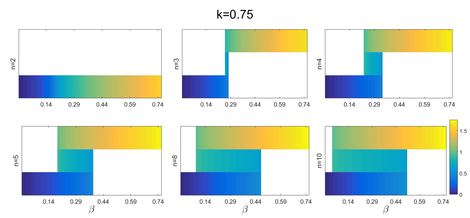Figure 1. Heatmaps showing the fixed points of a self-activating gene at different values of the cooperativity parameter. There are three bands corresponding to the three possible fixed points.

Or as lineplots where the unstable fixed points are shown by the red dotted lines, called by the command:

fcn_plot_bifurc_diff_n(roots_real_nonnegat_matr, beta_vals, n_vals,k_val,plot_pars)

and producing these plots: 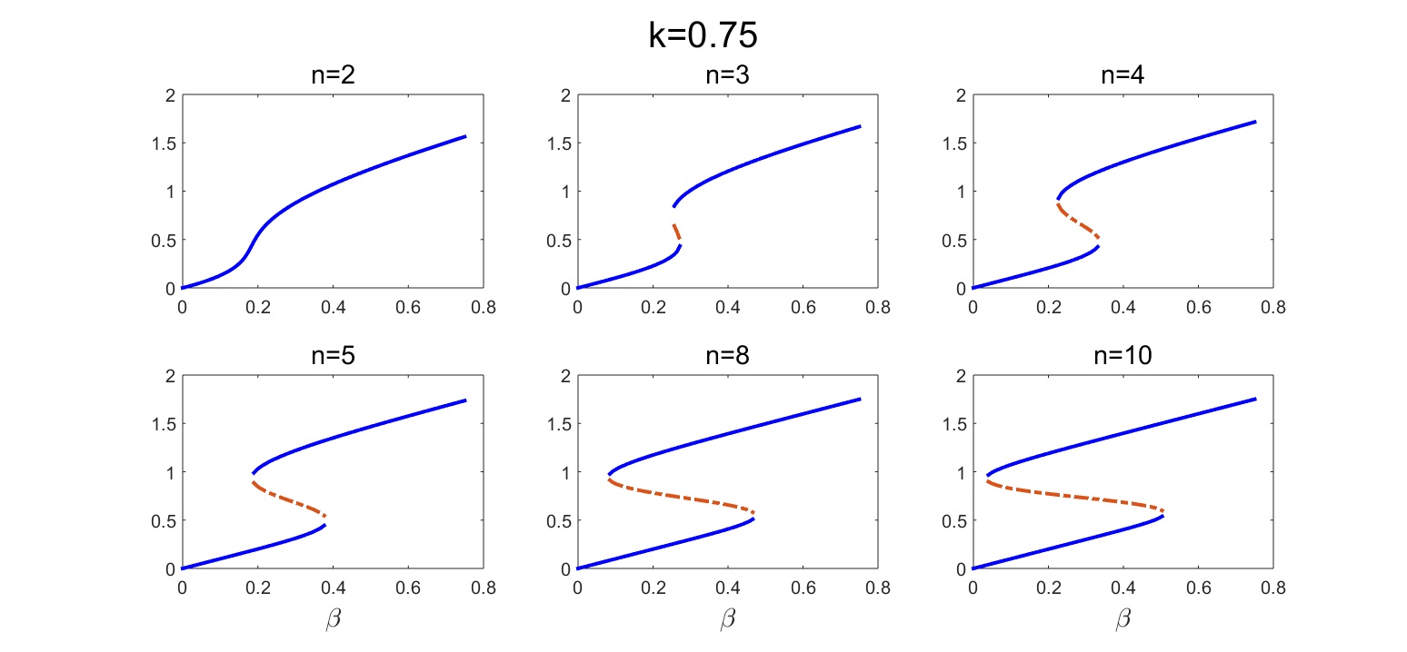Figure 2. Bifurcation plots for a self-activating gene at different values of the cooperativity parameter. Blue lines are stable fixed points, dashed red lines are unstable.

The lower threshold for the bistable range goes down while its extension grows with an increasing nonlinearity of the auto-activation.

Now, as it was shown by one of the first landmark papers [1] of modern (>2000) systems biology how two genes mutually inhibiting each other can lead to bistable behavior if the inhibition has a nonlinear (sigmoidal effect). In this [2] paper it was pointed out that if the auto-activation of these two genes already makes them bistable then coupling them can generate several stable fixed points.

To intuitively illustrate this point, before setting up a model, let’s call the two genes A and B and we visualize their nullclines as a function of the value of the other gene. Note that as we analyze the system in 2D now the basal production rate is a single value, we are not scanning through a range of values. Where the two nullclines intersect we have a global fixed point: both variables have 0 time derivatives at these intersection points.

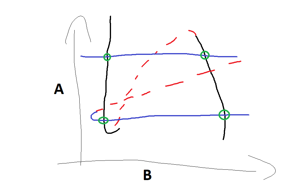
Figure 3: Sketch of intersecting nullclines

We can have up to 9 intersection points and 4 of them can be intersections of the stable branches of the nullclines, shown by the green circles, so these will be stable fixed points.

I implemented this two-dimensional system with adjustable parameters in MATLAB. First, I calculate the nullclines by polynomial root-finding.

The equations for the two genes are:
$\frac{dA}{dt} = \beta_A + f_A (1 + f_{BA}) - A$
$\frac{dB}{dt} = \beta_B + f_B (1 + f_{AB}) - B$

$f_A$ and $f_B$ are the self-activation functions, $f_{BA}$ is the inhibition mechanism from $B$ to $A$ and $f_{AB}$ vice versa. The basal production terms and the decay terms are as in eq. \ref{ode_autoact}.

Expanding the activation and inhibition functions the full equations are:
$\frac{dA}{dt} = \beta_A + \frac{A^n}{ A^n + k_{AA}^n } (1 + \frac{k_{BA}^n}{k_{BA}^n + B^n}) - A$
$\frac{dB}{dt} = \beta_B + \frac{B^n}{ B^n + k_{BB}^n } (1 + \frac{k_{AB}^n}{k_{AB}^n + A^n} ) - B$

Again, since we are (first) solving for the stationary solutions we can rearrange the equations to polynomial form and for each equation treat the other variable as a parameter to calculate the nullclines. This is done by calling the function fcn_nullclines_double_inhib. We need to specify the range of values for the two variables where the nullclines are calculated and also the six parameters $[n,k_{AA},k_{BA},\beta_a,k_{BB},k_{AB},\beta_b]$.

n=4;
kAA=3/4; kBB=3/4;
beta_a=1/4; beta_b=1/4;
kBA=1/2; kAB=1/2;
params = [n,kAA,kBA,beta_a,kBB,kAB,beta_b];
maxval_B=2.25; logvals=logspace(-2,log10(maxval_B),200);
linvals=linspace(0.01,maxval_B,300);
B_vals=[0 linvals]; A_vals=[0 linvals];
[real_nonnegroots_f1,real_nonnegroots_f2] = fcn_nullclines_double_inhib(A_vals,B_vals,params);

Polynomial rootfinding is rather fast, for 200 input values, the calculation takes 35 seconds on my laptop (CPU @ 2.50GHz, 2601 Mhz, 2 Core(s)).

Next we can visualize the nullclines and their intersections that are the fixed points of the model by the function fcn_plot_double_inhib:

parnames='$[n, k_{AA}, k_{BA},\beta_a, k_{BB},k_{AB},\beta_b]=$';
legend_str={'dA/dt=0,stable','dA/dt=0,unstable','dA/dt=0,stable'};
plot_pars={22,3,5,parnames,legend_str,0.02};
fcn_plot_double_inhib(B_vals,real_nonnegroots_f1,A_vals,...
    real_nonnegroots_f2,params,plot_pars,'vectorfield')

The flag ‘vectorfield’ tells the function to evaluate the algebraic equations that are the right-hand side of the differential equations showing the value of time-derivatives at that point of the coordinate system.

For a parameter set with basal production rates falling within the bistable region of the bifurcation plot on Figure 2 for $n=4$ both variables have nullclines with 3 branches across the entire range.

Figure 4: Inhibition-coupled bistable genes, parameter set resulting in 4 stable fixed points. Green and blue lines showing the stable branches of the nullclines, dash-dotted thinner lines the unstable ones. Vector field showing the derivatives of the two state variables.

The stable branches are shown by thicker markers (green and blue) and the unstable ones by dashed-dotted thinner lines. The intersections of the stable branches have to be the fixed points of the system.
It is interesting to visualize this as well and also the basins of attractions of the fixed points. To do this we numerically integrate the ODEs from a grid of initial conditions and store the solutions in the cell trajectories:

initvals=linspace(0,2.25,16); tspan=0:0.01:20; initvals_perms=permn(initvals,2);
options = odeset('RelTol',1e-4); % ,'AbsTol',at
trajectories=cell(1,size(initvals_perms,1));

for initv1=1:size(initvals_perms,1)
    disp(initv1/size(initvals_perms,1)); x0=initvals_perms(initv1,:);
    [t,x]=ode45(@(t,x)fcn_odes_double_inhib(t,x,params),tspan, x0);
    trajectories{initv1}=x;
end

For the parameter set above the trajectories look like this:

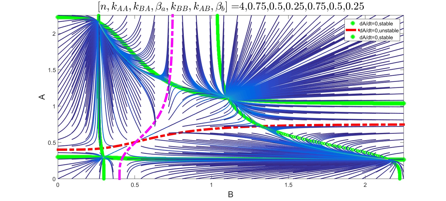Figure 5: Inhibition-coupled bistable genes: parameter set resulting in 4 stable fixed points. Trajectories from different initial conditions converging to one of the four fixed points.

We can see how the unstable branches are the ‘frontiers’ of the basins of attraction.

An interesting case is a parameter set when the nullcline don’t just intersect at given points, but overlap along a whole section:

Figure 6: Inhibition-coupled bistable genes, parameter set resulting in overlapping nullclines yielding fixed points along the overlapping section.

In this case the overlapping section of the nullclines are all fixed points, so trajectories in the basin of attraction converge to different points of this line. This means (I think) there are infinitely many stable solutions that converge on the points of this line section in this region of the phase space. It would be interesting to explore what this means in terms of the polynomials.

An interesting question is what if we couple more than 2 bistable components. Would we get multistability with more than 4 fixed points? I might explore this question in a future post.

The script with its functions are available on GitHub and they can be downloaded and used in MATLAB.

1. [1]T. S. Gardner, C. R. Cantor, and J. J. Collins, “Construction of a genetic toggle switch in Escherichia coli,” Nature, vol. 403, no. 6767, p. 339, 2000.
2. [2]M. Lu, M. K. Jolly, R. Gomoto, B. Huang, J. Onuchic, and E. Ben-Jacob, “Tristability in cancer-associated microRNA-TF chimera toggle switch,” The journal of physical chemistry B, vol. 117, no. 42, pp. 13164–13174, 2013.

Written on December 25, 2019

[ systems-biology  nonlinear-dynamics  multistability  kinetics  complex-systems  ]