Dynamic behavior of sequentially determined values

In my previous post I discussed a simple model of sequentially defined prices of production. These production prices for any good are defined as the good’s input cost (wages + non-labour costs) plus a markup equal to the rate of profit/surplus labor in the entire (two department) economy. As I discussed this model eventually converges to a stationary solution that is identical of the algebraic system of equations with identical input and output prices, ie. $\mathbf{p} = \mathbf{p}(\mathbf{A} + w \mathbf{l})(1+r) \tag{1}\label{simul_val}$

The system of difference equations for (more than one) prices of production had a nonlinear term due to profit rate equalization, ie. redistribution of value produced in the different sectors: $\mathbf{p}_{t+1} = \mathbf{p}_t (\mathbf{A} + w \mathbf{l}) (1 + \frac{ \mathbf{l} \mathbf{X} - \mathbf{p}_t w \mathbf{l} \mathbf{X} }{ \mathbf{p}_t (\mathbf{A} + w \mathbf{l}) \mathbf{X} } ) = \mathbf{p}_t (\mathbf{A} + w \mathbf{l}) \frac{ ( \mathbf{p}_t \mathbf{A} + \mathbf{l}) \mathbf{X} }{ \mathbf{p}_t (\mathbf{A} + w \mathbf{l}) \mathbf{X} } \tag{2}\label{unit_price_dynam_explicit}$

It is obvious that in the case of a model with only one good, so if $A$, $l$, $X$ are scalars, not matrices/vectors, the nonlinearity drops out and the system simplifies to $p_{t+1} = p_t a + l$, that has an explicit solution, which is:

$p_{t} = p_0 a^t + l \sum_{i=0}^{t-1} a^i = p_0 a^t + \frac{l}{1-a} (1-a^t)$,

which for $a<1$ (meaning there is a physical surplus) converges to $p^* = \frac{l}{1-a}$. In this case there is no redistribution of added value through prices of production, so value and price are the same, equaling to the price of inputs plus the incorporated labour.

Since it is more interesting to work with the more general case of multiple goods/sectors, but without the non-linearity, I will look at the dynamic behavior of values instead of prices of production, following an exchange between Duménil&Lévy (D&L) and P. Giussani around 2000 [1] [2].

When I write the value of a particular good, I mean the value of its inputs plus the amount of (socially necessary) labour directly embodied in it, ie. using a sequential definition
$\Lambda_t = \mathbf{A} \Lambda_{t-1} + \mathbf{L}_t \tag{3}\label{dynamic_values}$

or in the simultaneous description (dropping time subscripts):

$$\Lambda = \mathbf{A} \Lambda + \mathbf{L} \tag{4}\label{simult_values}$$

where again $L$ is the column vector of labour values, $A$ the input-output matrix, and $\Lambda$ the column vector of unit values.

The solutions for the unit values are then for simultaneous values:

$$\Lambda = (\mathbf{I} - \mathbf{A})^{-1} \mathbf{L} \tag{5}\label{simult_values_sol}$$

and sequentially determined values:

$$\Lambda_t = \mathbf{A}^{t} \Lambda_0 + (\mathbf{I} - \mathbf{A})^{-1} (\mathbf{I} - \mathbf{A}^{t} ) \mathbf{L} \tag{6}\label{dynamic_values_sol}$$

Since it is assumed (elements of) $A<1$ (otherwise we would have shrinking reproduction), therefore $\lim\limits_{t \to \infty}\Lambda_t = \Lambda^{* } = (I-A)^{-1} L$, same as the simultaneous equation \ref{simult_values_sol}. For this reason it was argued by Stamatis [3] [4] that the sequential formalism is simply an iterative calculation procedure to solve the algebraic equation of \ref{simult_values_sol}, and not a model of economic dynamics. I will address this question later, first I will explore some dynamic properties of this formalism, independent of its interpretation.

It was pointed out by D&L that in the sequential formalism it is possible to have growing labour productivity (falling labour inputs per unit of goods) with growing unit values. Specifically, if instead of a constant $L$, it is now a function of time:

$L_t = \alpha + \beta \gamma^t$,

with $0<\gamma<1$, that is $L$ will be monotonically decreasing with time, falling to $\alpha$ eventually (the coefficients are column vectors).

The explicit solution for sequential values is then:

$$\Lambda_t = A^t \Lambda_0 + (I - A)^{-1} (I-A^t) \mathbf{\alpha} + (A - \gamma I)^{-1} (A^t - \gamma^t I) \mathbf{\beta} \tag{7}\label{dynamic_values_sol_L_t}$$

if $\gamma$ is a scalar, otherwise the last term is $(A^t - \left< \gamma^t \right> I ) \beta$, with $\left< \gamma \right>$ being the diagonal matrix from $\gamma$. Since the $A^t$ and $\gamma^t$ terms are shrinking to zero with time, the equilibrium solution is:

$\Lambda^{* } = (I-A)^{-1} \mathbf{\alpha}$,

again the same as in the simultaneous description.

D&L point out that if the initial value $\Lambda_0 < \Lambda^{* }$, then $\Lambda^{t}$ will rise, converging to the equilibrium from below, even though the labour content is falling. D&L refer to this as a ‘productivity paradox’. In fact, the behavior of sequential values is even more complex. In equation \ref{dynamic_values_sol_L_t} there are exponential terms both in $A$ and $\gamma$ suggesting the behavior can be non-monotonic. This is in fact what happens with certain parameter sets as shown by the numerical examples below.

The parameter set used was: $\mathbf{\alpha}= [0.2; 0.4], \mathbf{\beta}= [0.3; 0.1], \mathbf{\gamma}= [0.9; 0.8], \mathbf{A} = \begin{bmatrix} 2/3 & 1/3 \\ 1/6 & 1/2 \\ \end{bmatrix}$

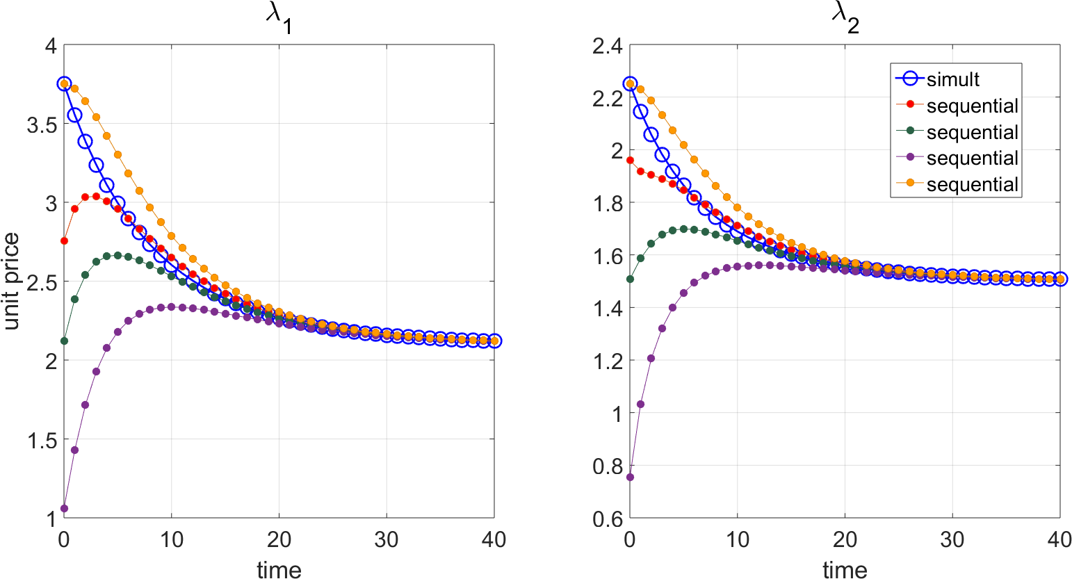Figure 1: Non-monotonic dynamics of sequential values with increasing productivity

This non-trivial and somewhat puzzling feature comes about because of two dynamical terms that can be seen in equation \ref{dynamic_values_sol_L_t}: one coming from the input values of the previous period and the other from labor productivity. If the initial input values are far from the stationary value (of the simultaneous equations with that level of productivity) then it can take several iterations until the falling labor content becomes the dominant term, and this can result in non-monotonic behavior.

For the one-good case, it is easier to see the conditions for this. In this case the difference $\epsilon$ between any two consecutive steps is:

$$\epsilon = \left(\lambda_0 - \frac{\alpha}{1-a} + \frac{\beta}{a-\gamma} \right) a^t \left(1-\frac{1}{a} \right) + \left(- \frac{\beta}{a - \gamma} \right) \gamma^t \left(1-\frac{1}{\gamma} \right)$$

Denoting the difference between the initial and stationary value $\Delta = \lambda_0 - \frac{\alpha}{1-a}$, and after some rearrangements, the condition for non-monotonic behavior is:

• $\Delta < \frac{\beta}{a-\gamma} \left( \frac{\gamma}{a}^{t-1} \frac{\gamma-1}{a-1} -1 \right)$, if $\Delta >0$ (increasing unit values for $\lambda_0 > \lambda^*$)

• $\Delta > \frac{\beta}{a-\gamma} \left( \frac{\gamma}{a}^{t-1} \frac{\gamma-1}{a-1} -1 \right)$, if $\Delta < 0$ (decreasing unit values for $\lambda_0 < \lambda^*$)

As the numerical example above shows this can be satisfied in both cases.

Is this behavior of sequential values «paradoxical»? No matter how we answer this question, it certainly would be an exaggeration to claim that what we see here is - even an extremely simplified - model of economic dynamics. The technical coefficients of the system are defined independently from values, there are no feedback effects, and yet the system shows relatively complicated dynamic behavior already, depending on its initial value. This is not due to endogenous technical change or of disequilibrium between supply and demand, but simply to the dependence on the previous state.

Yet this can also be seen as an interesting feature of the sequential model, in contrast to the simultaneous one, namely that the periods are connected: the output price/value of one period is the input of the next. This suggests that it can be used in a dynamical model of the circuit(s) of capital [5]. If we have only one circuit per sector like above, this assumes that all capitals in that sector are synchronized, which is clearly not the case in reality. But if they are not synchronized, the formalism would have to be more complex. When one circuit of capital is in the phase of production others are releasing new products to the market, which can devalue the inputs. Therefore the value of inputs would not equal their original value, but would be - intuitively - some weighted average of past values of the inputs used by the individual circuits. In my next posts I want to address this question of connecting a model of the circuit of capital with these different methods of value calculation.

1. [1]P. Giussani, “Dynamic and Static Marxian Values,” Political Economy, vol. 3, no. 3, pp. 5–19, 1998.
2. [2]G. Dumenil and D. Levy, “The Conservation of Value. A Rejoinder to Alan Freeman,” Review of Radical Political Economics, vol. 32, no. 1, pp. 119–146, 2000.
3. [3]G. Stamatis, “Some remarks upon the article of Alan Freeman ’Marx without equilibrium,’” Political Economy, vol. 3, no. 3, pp. 21–23, 1998.
4. [4]G. Stamatis, “The so-called Temporal Single System (TSS) the so-called Standard Simultaneous Methodology (SSM) and the correct definition of labour values,” Political Economy, vol. 3, no. 5, pp. 23–44, 1999.
5. [5]D. K. Foley, “Realization and Accumulation in a Marxian Model of the Circuit of Capital,” Journal of Economic Theory, vol. 28, no. 2, pp. 300–319, 1982.

Written on March 2, 2019

[ political-economy  economic-models  classical-political-economy  marxian-economics  transformation-problem  ]